28.21 Choosing Dimensions

REVIEW

# Load packages from the local library into the R session.

library(rattle)   # For the weatherAUS dataset.
library(ggplot2)  # To generate a density plot.

# Identify cities of interest.

cities <- c("Canberra", "Darwin", "Melbourne", "Sydney")

# Generate the plot.

weatherAUS %>%
  subset(Location %in% cities & ! is.na(Temp3pm)) %>%
  ggplot(aes(x=Temp3pm, colour=Location, fill=Location)) +
  geom_density(alpha=0.55)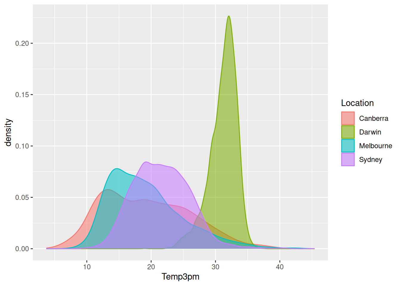

Often a bit of trial and error is required to get the dimensions right. Notice though that increasing the fig.width= as we did for the previous plot, and/or increasing the fig.height=, effectively also reduces the font size. Actually, the font size remains constant whilst the figure grows (or shrinks) in size. Sometimes it is better to reduce the fig.width or fig.height to retain a good sized font.

The above plot was generated with the following knitr (Xie 2025) options.

<<myfigure, echo=FALSE, fig.height=3.5}
... R code ...
@

References

———. 2025. Knitr: A General-Purpose Package for Dynamic Report Generation in r. https://yihui.org/knitr/.

---

If you find this curated material useful then you can consider a donation to support it's ongoing availability and give you access to the PDF version of this book. The material has been scoped up by Generative AI without permission or any kind of recompense so do consider a donation if you can afford it. Unlike Generative AI your access to this materials is freely given. Desktop Survival Guides include Data Science, GNU/Linux, and MLHub. Books available on Amazon include Data Mining with Rattle and Essentials of Data Science. Togaware has a 30 year tradition of making popular open source software which includes sold privacy preserving productivity apps, rattle, wajig, and mlhub. Hosted by Togaware, a pioneer of free and open source software since 1984. Copyright © 1995-2022 Graham.Williams@togaware.com Creative Commons Attribution-ShareAlike 4.0