11.11 Bar Chart Flipped Colour Mean Confidence Intervals
20200822
ds %>%
filter(location %in% (ds$location %>% unique %>% sample(20))) %>%
mutate(location=factor(location,
levels=location %>% unique() %>%
sort() %>% rev())) %>%
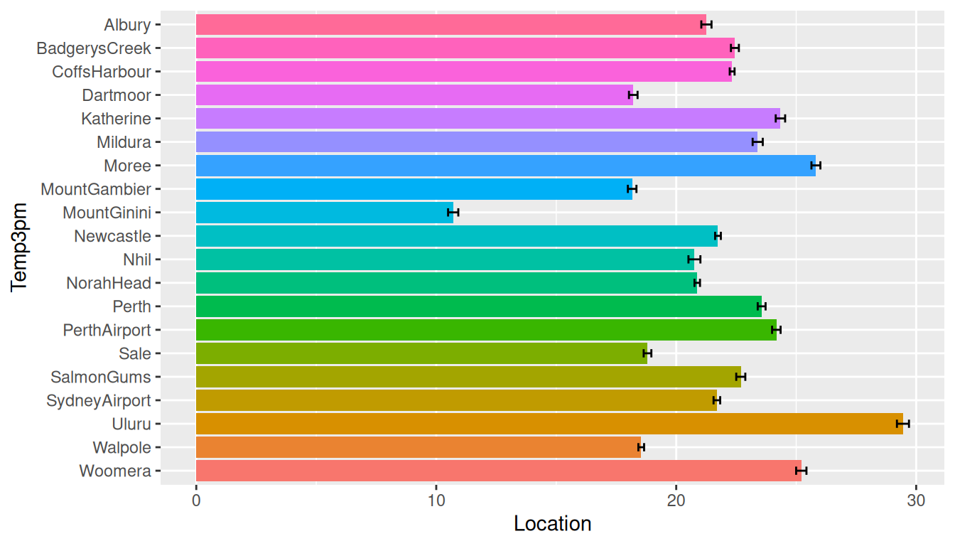
ggplot(aes(location, temp_3pm, fill=location)) +
stat_summary(fun="mean", geom="bar") +
stat_summary(fun.data="mean_cl_normal", geom="errorbar", width=0.35) +
theme(legend.position="none") +
labs(x=vnames["temp_3pm"], y=vnames["location"]) +
coord_flip()Various annotations can be added to plots. In this example we include a confidence interval around the average values.
Exercise: review the confidence intervals—do they make sense?
Your donation will support ongoing availability and give you access to the PDF version of this book. Desktop Survival Guides include Data Science, GNU/Linux, and MLHub. Books available on Amazon include Data Mining with Rattle and Essentials of Data Science. Popular open source software includes rattle, wajig, and mlhub. Hosted by Togaware, a pioneer of free and open source software since 1984. Copyright © 1995-2022 Graham.Williams@togaware.com Creative Commons Attribution-ShareAlike 4.0