11.25 Box Plot

20240728

ds %>%
  mutate(year=factor(format(ds$date, "%Y"))) %>%
  ggplot(aes(x=year, y=max_temp, fill=year)) +
  geom_boxplot(notch=TRUE) +
  stat_summary(fun=mean, geom="point", shape=8) +
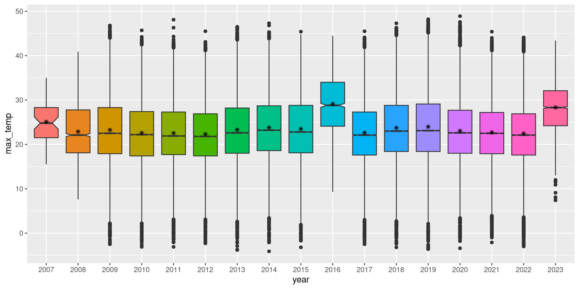
  theme(legend.position="none")

A box plot provides a graphical overview of how the values of a numeric variable are distributed. It is useful for quickly ascertaining the skewness of the distribution of the data. Also known as a box and whiskers plot it presents visually the median (the second quartile or 50th percentile) as the thicker horizontal line within the box. The box itself then extends to the lower (the first quartile or 25th percentile) and upper quartiles (the third quartile or the 75th percentile) which delimit one quarter of the dataset each, and hence the box itself represents half the dataset. The extent of the box is known as the interquartile range.

The vertical lines extend from the box to the maximum and minimum data points that are no more than 1.5 times the interquartile range from the median. Outliers (points further than 1.5 times the interquartile range from the median) are then individually plotted. The mean is also added to the plot here and displayed as the asterisk.

The notches in the box, around the median, indicate a level of confidence about the value of the median for the population in general. It is useful in comparing the distributions that are presented in the chart and allows us to readily see which distributions have significantly different medians. These are where the notches do not overlap.

In our example here we add colour to improve the visual appeal of the plot and to more readily separate the different values for the year. Using fill= we also turn off the otherwise included legend.

Through this plot we can observe the overall change in the maximum temperature over the years. Notice the first and last plots might reflect truncated data and the plot for 2016 is an outlier. These observations might lead us to review the data before we make any significant statements about the data.

---

Your donation will support ongoing availability and give you access to the PDF version of this book. Desktop Survival Guides include Data Science, GNU/Linux, and MLHub. Books available on Amazon include Data Mining with Rattle and Essentials of Data Science. Popular open source software includes rattle, wajig, and mlhub. Hosted by Togaware, a pioneer of free and open source software since 1984. Copyright © 1995-2022 Graham.Williams@togaware.com Creative Commons Attribution-ShareAlike 4.0