|
ds %>%
ggplot(aes(x=date, y=max_temp)) +
geom_point(alpha=0.05, shape=".") +
geom_smooth(method="gam", formula=y~s(x, bs="cs")) +
facet_wrap(~location) +
theme(axis.text.x=element_text(angle=45, hjust=1)) +
labs(x=vnames["date"], y=vnames["max_temp"])
Partitioning the dataset by a categoric variable reduces the blob
effect for big data. The plot uses location as the faceted
variable to separately plot each location's maximum temperature over
time. Notice the seasonal effect across all plots, some with quite
different patterns.
The plot uses facet_wrap() to separately plot each
location. Using ggplot2::geom_point() with alpha=
reduces the effect of overlaid points. Using smaller dots on the plots
by way of shape= also de-clutters the plot significantly and
improves the presentation and emphasises the patterns. The x axis tick
labels are rotated 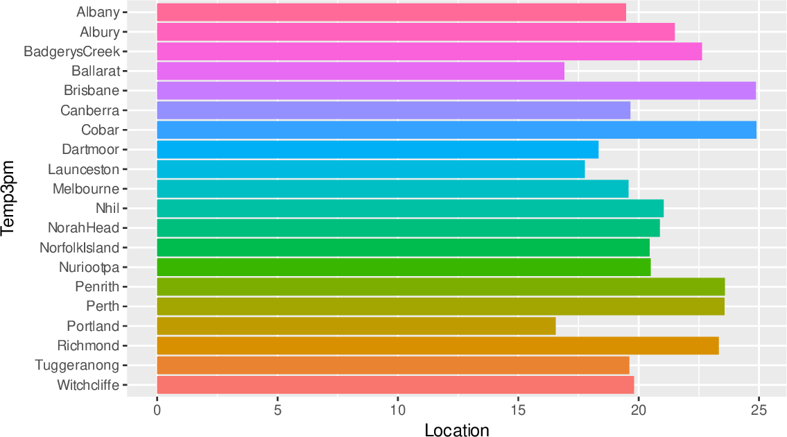 using angle=45 within
ggplot2::element_text() to avoid the labels overlapping. The
hjust=1 forces the labels to be right justified. using angle=45 within
ggplot2::element_text() to avoid the labels overlapping. The
hjust=1 forces the labels to be right justified.
| 


![\includegraphics[width=\textwidth]{figures/onepager/ggplot2:temp_changes_over_time-1}](img48.png)